Standard Deviation Corrector
Corrects bias in sample SD displayed by a chronograph.
(Valid for all Normally distributed variables, like muzzle velocity.)
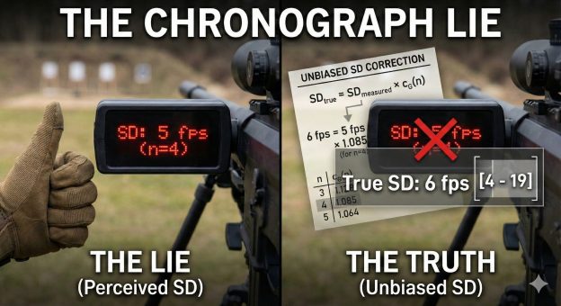
If you spend time on shooting forums or Instagram, you’ve seen the photos: A chronograph screen proudly displaying a Standard Deviation (SD) of muzzle velocity under 5 fps. A caption praising a specific powder or intricate reloading process.
If you spend time chronographing your own loads you might notice an irritating tendency for the SD to increase the more shots you take. This is not an illusion: the formula current chronographs use for Standard Deviation is biased. The bias is greatest for the smallest sample sizes.
Estimated Standard Deviation is mathematically biased to be low, and significantly so for small samples.
The true standard deviation of a lot of ammunition is a fixed number that doesn’t depend on how many rounds you shoot.1 But nobody shoots an entire lot of ammunition to evaluate it. Instead, we shoot a small sample to estimate its characteristics and determine whether to buy (or load) the remainder of the lot. And when we’re paying for each shot, there’s a strong incentive to make up our mind with as few shots as possible.
The Small Sample Trap
Most shooters live in “small sample space.” We shoot 3 or 5 rounds to check a load. We look at the SD reported by the chronograph, and if we see a low number we’re happy and we move on.
Here is the problem: The formula used to calculate “Sample Standard Deviation” contains a mathematical bias. If we compute the average of the estimated SD over a number of experiments, we will find that it is always lower than the true SD. The smaller the sample size (n), the larger the understatement of the SD. (Do this often enough and you instinctively know this. If paying for each round weren’t enough motivation to keep sample sizes small, the fact that SD creeps up as you keep shooting only adds to that.)
The Bias Correction Factor
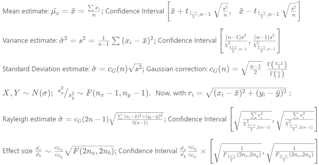
Fortunately, because muzzle velocity is Normally distributed, we can correct this bias. We only need to multiply the (biased) SD by a correction factor, and that factor depends only on the number of shots used to estimate the SD. The formula for the correction factor cG(n) may look intimidating,2 but as you can see from the following table it really only matters for small sample sizes. You can look it up here, or use the calculator at the top of this post.
| Number of shots (n) | Multiply by (correction factor) |
|---|---|
| 2 | 1.25 |
| 3 | 1.13 |
| 4 | 1.09 |
| 5 | 1.06 |
| 6 | 1.05 |
| 7 | 1.04 |
| 8 | 1.04 |
| 9 | 1.03 |
| 10 | 1.03 |
A Real World Example
Let’s say you head to the range with a promising new load. You fire 4 shots and your chronograph reports an SD of 5.5 fps. Not bad! But now you know that you have to correct that, so:
- Look up the correction factor for n=4: It’s 1.09.
- Multiple the reported SD by that factor: 5.5 × 1.09 = 6.0.
Now you know the unbiased estimate of the SD of the new load: 6.0 fps.
Confronting Reality with Confidence Intervals
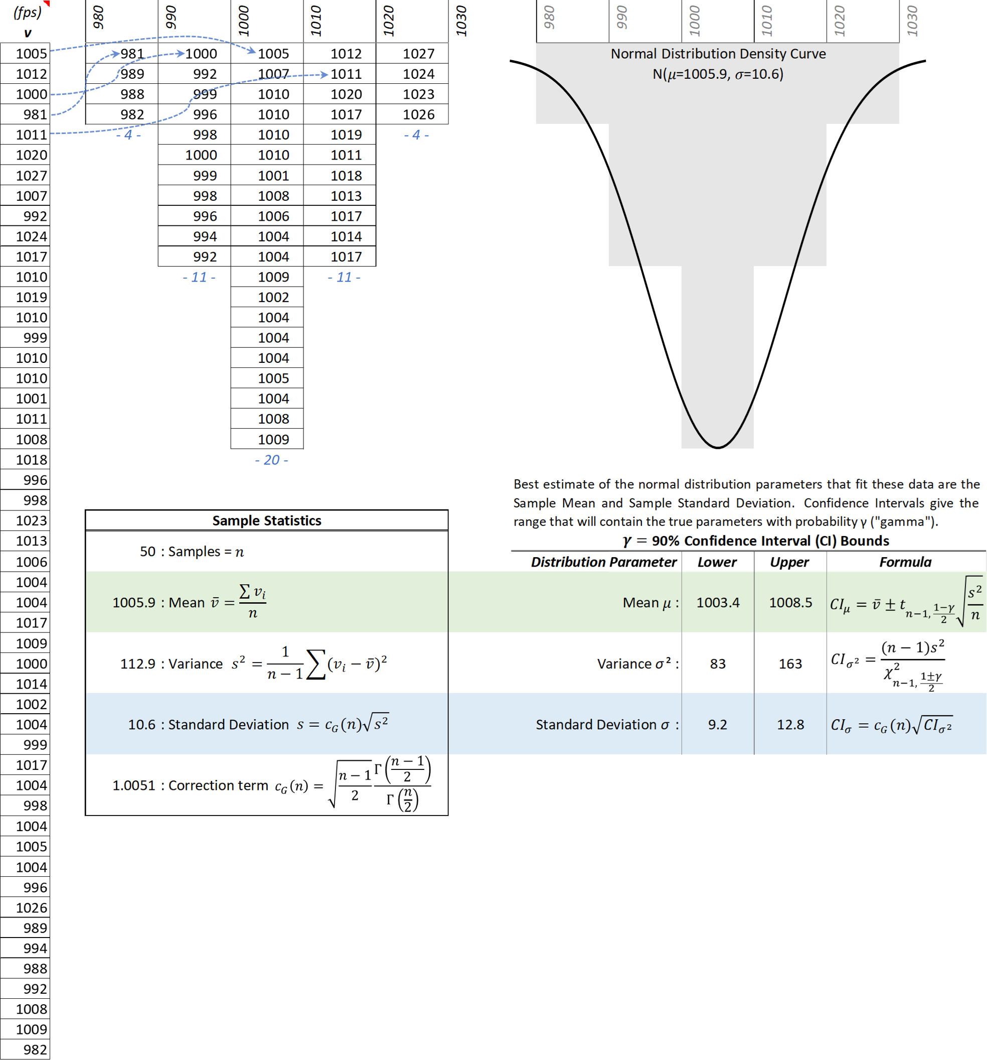
Correcting for bias gives us an unbiased estimate, but it doesn’t tell us how good that estimate is. For that we have the Confidence Interval (CI). The calculator at the top of this page will give you not only the unbiased estimate but also the 90% Confidence Interval. And if you begin to look at that you will understand why only the most disciplined shooters embrace the hard reality of statistics: Using the same example (4 shots, corrected SD of 6.0 fps), the statistical uncertainty is high. The 90% Confidence Interval for that load is actually [3.4, 16.0].
That means the “5.5 fps SD” bragging rights sample is statistically consistent with an ammo lot that has an SD as high as 16 fps.
How do we reduce statistical uncertainty? There’s no substitute for sample size. In this case, we can halve the Confidence Interval by taking 4 more shots. Try it in the calculator: 8 shots reporting an SD of 5.8 gives a corrected SD of 6.0 fps but now with a 90% CI of [4.1, 10.3]. With those data it’s reasonable to believe the true SD is in single digits.
Want to dig in further? I set up Google Sheets here to calculate detailed statistics for shooters while making it easy to inspect the formulas and math behind them.
The Takeaway
A true standard deviation of less than half a percent (e.g., single digit SD for high-velocity guns) is a remarkable achievement. But naive statistics and small sample sizes lull us into a false sense of precision.
Next time you see an exceptionally low SD, check the sample size. If you can count the shots on one hand, you can bet the house that the true SD is higher.
- Unless you introduce some variance. For example, if you continue to shoot through an overheating barrel then muzzle velocity will decrease. If you continue to shoot through an excessively fouled barrel then muzzle velocity will increase. ↩︎
- The correction term for a group size n can be computed using the following spreadsheet formula:
=EXP(GAMMALN((n-1)/2) - LN(SQRT(2/(n-1))) - GAMMALN(n/2))↩︎


