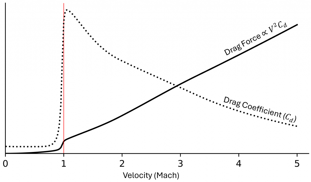
As soon as a bullet leaves the barrel of a gun it encounters air resistance, which slows it down. So in order to compute a ballistic trajectory in an atmosphere we need an accurate model of aerodynamic drag. Here’s an example of the drag curve for one common bullet:

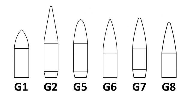
Back when ballistic calculations were done with tables and slide rules, bullets were related (via Ballistic Coefficient, a.k.a BC) to one of a handful of standard projectile shapes for which the drag curve had been experimentally tabulated. Here are the shapes:

In fact, prior to the turn of the century, sporting bullet manufacturers only published ballistic coefficients that referenced G1, and ballistic calculators didn’t bother with drag models other than G1. This was not ideal because many long-range rifle bullets are shaped more like G7, as can be seen in this photo of bullets that I have tested:

One hack for this problem was to break up the drag model into velocity regions and use a different ballistic coefficient for each. For example, a 250gr .338 OTM bullet has a G1 BC of 0.55 for speeds below Mach 1.5, 0.60 up to Mach 2, and 0.63 above. This produces more accurate trajectories than using a single G1 BC for all speeds.

In recent decades manufacturers have begun to publish ballistic coefficients for the G7 model as well. This same period has seen growing interest in precision shooting sports that reward first-round hits at varied and long ranges. And people have discovered that we can do even better than G7 for many bullets. Using the multiple-coefficient approach, that same 250gr .338 bullet has a G7 BC of 0.305 below Mach 1.5, 0.31 up to Mach 2, and 0.32 above. So not a huge difference from using a single G7 BC of 0.314, but it is measurable at extended ranges – in this case it’s more than 5″ of vertical error at 1000 yards.

Why are we still dealing with piecewise approximations to drag models? Getting a precise drag curve for a specific bullet is not too difficult: Ranges equipped with radar and/or microphone arrays can track the speed of test shots over their entire trajectory. It doesn’t take much data: The standard drag curves cover speeds from 0 to Mach 5 using only 80 points. It’s not a big ask for bullet manufacturers to record and publish drag data for each bullet design they make. (For example, Hornady uses radar to measure drag curves for their bullets, but so far they have only made those available through their closed-source ballistic calculator.)