Category Archives: Ballistics

Standard Drag Models and Ballistic Coefficients

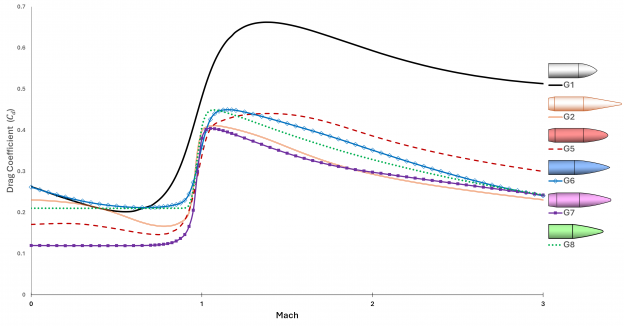
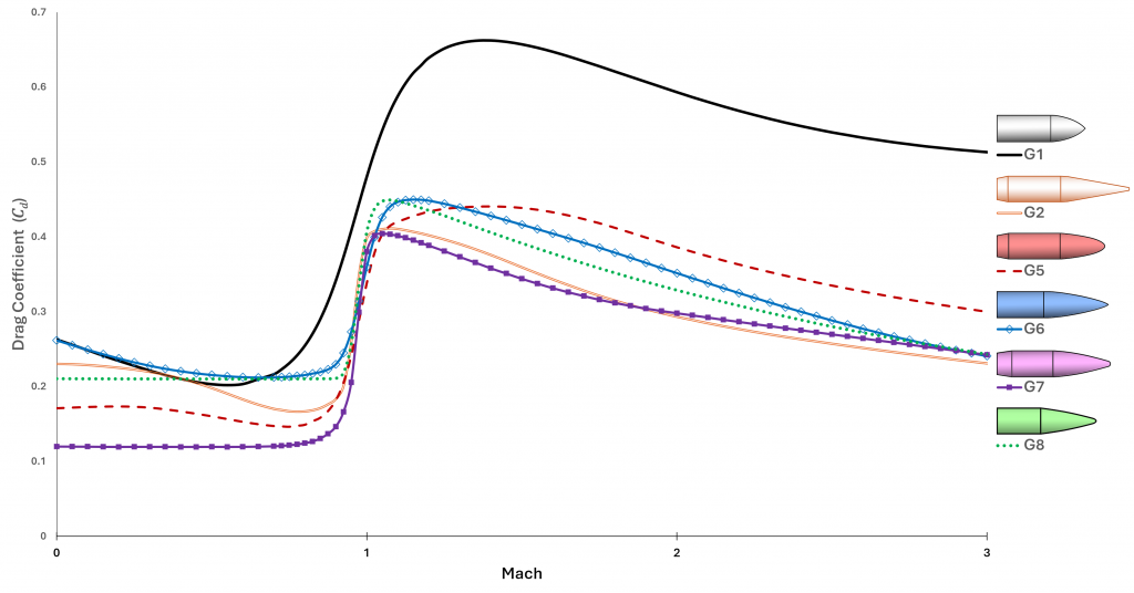
The last post mentioned the standard ballistic drag curves. Here is a chart of them for speeds up to Mach 3:

Standard Ballistic Drag Curves for speeds from 0 to Mach 3.

This chart reveals a few quirks of the standard drag models.  First is that G1 is not very precise in the transonic region (i.e., about Mach 1).  The reality of the sound barrier is reflected in the other curves, where drag hits a steep cliff that doubles or triples the subsonic drag coefficient.  The more gentle slope of the G1 curve is a result of 19th century ballisticians failing to adjust aggregate test data for variations in the speed of sound.

Looking at the low subsonic region we find another strange artifact: several of the curves show an increase in drag as speed goes to zero.  The reality is that drag should be virtually constant across low subsonic speeds.  I asked Jeff Siewert what is going on here and he explained: Back in the day, the test ranges reported what they observed, and at those low speeds the projectiles (especially G2) were likely encountering dynamic instability that increased their yaw.  So those segments reflect an increasing aerodynamic cross-section, not the (constant) drag that would be seen in stable, nose-forward flight.

Example: .308 OTM

G7 vs 168gr .308 OTM profiles

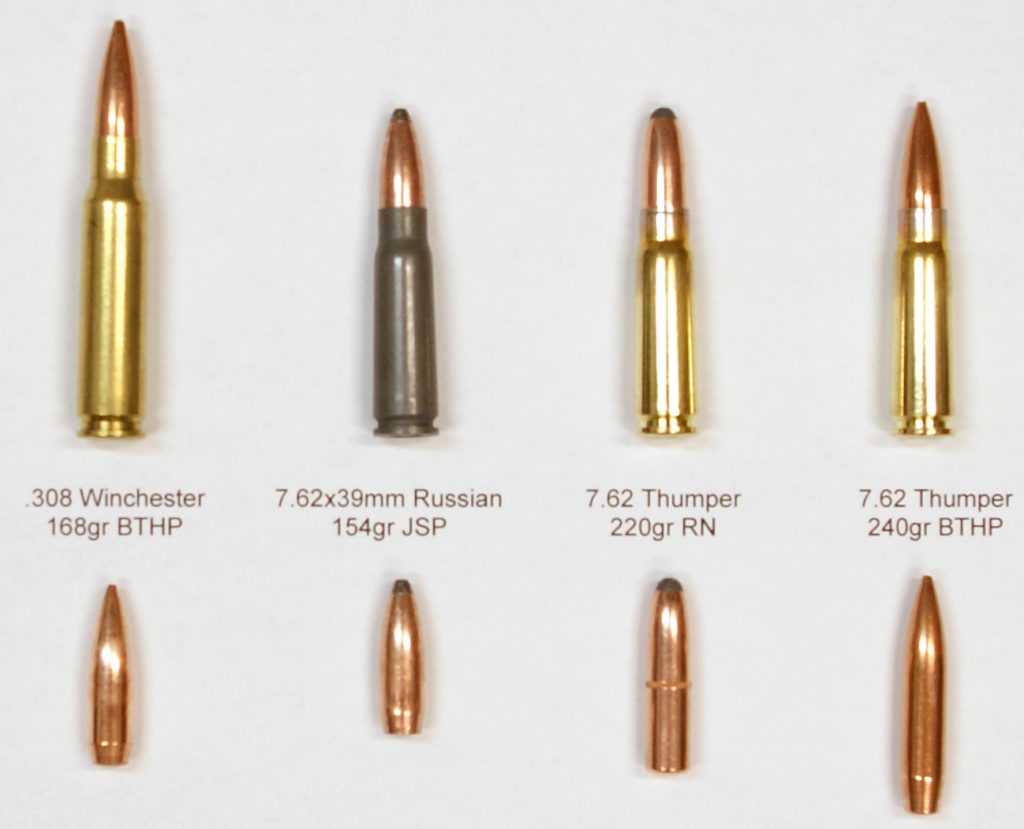
Let’s look at a typical rifle bullet: the 168gr .308 BTHP (boat-tail hollow-point), a.k.a. open-tip match (OTM). The profile of this bullet looks very close to the G7 standard projectile, as shown in this image with scaled profiles of the two:

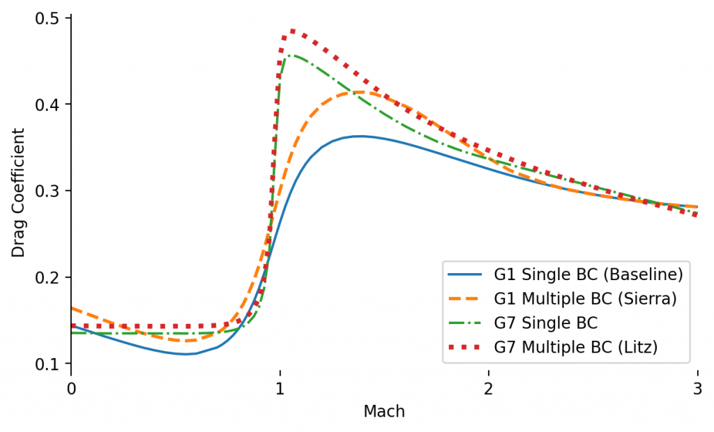
Manufacturers of this bullet still list a Ballistic Coefficient (BC) of 0.462 for use with the G1 drag model. A few decades ago, in an effort to improve trajectory predictions, Sierra published multiple G1 BCs for different velocity ranges: 0.462 above 2600 fps, 0.447 above 2100 fps, 0.424 above 1600 fps, and 0.405 below that. Eventually Berger began to publish G7 BCs, and this bullet is often quoted with a G7 BC of 0.224. A decade ago Bryan Litz began publishing detailed drag models for rifle bullets. For Sierra’s version of this bullet he lists multiple G7 BCs: 0.226 above 3000fps, 0.222 at 2500fps, 0.214 at 2000fps, and 0.211 below 1500fps. Here is a chart of the drag curves resulting from each of these variations:

Drag curves for different ballistic coefficients for the Sierra 168gr .308 OTM bullet.
Drag curves for the Sierra 168gr .308 OTM bullet.

Long-Range Consequences

How meaningful are these differences? I ran the trajectory for each model using a muzzle velocity of 3000fps, zeroed at 500 yards. Here are the drops on the baseline (G1) trajectory, and then the additional drop when using each of the other drag curves:

Baseline (G1)
Drop: Difference from Baseline
Distance (yards)Drop (inches)G1 MultiG7G7 Multi
500 0 0.1 0.6 0.6
1000233 8.710.3 16.3
150096278.595.9142.5

So there’s not a meaningful difference until we’re looking at ranges closer to 1,000 yards. At longer ranges, however, the vertical error from the inferior models is measured in feet!

Ballistic Drag Models

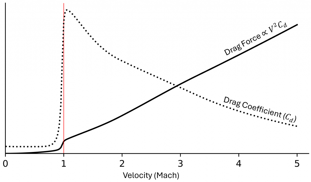
As soon as a bullet leaves the barrel of a gun it encounters air resistance, which slows it down. So in order to compute a ballistic trajectory in an atmosphere we need an accurate model of aerodynamic drag. Here’s an example of the drag curve for one common bullet:

Drag force and drag coefficient for .308 OTM bullet, using the G7 model.
Drag vs velocity for a standard .308 bullet (using G7 model)

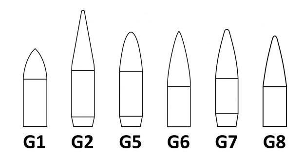
Back when ballistic calculations were done with tables and slide rules, bullets were related (via Ballistic Coefficient, a.k.a BC) to one of a handful of standard projectile shapes for which the drag curve had been experimentally tabulated. Here are the shapes:

Projectile shapes used for standard ballistic drag models

In fact, prior to the turn of the century, sporting bullet manufacturers only published ballistic coefficients that referenced G1, and ballistic calculators didn’t bother with drag models other than G1. This was not ideal because many long-range rifle bullets are shaped more like G7, as can be seen in this photo of bullets that I have tested:

,30 and ,22 bullets tested by David Bookstaber

One hack for this problem was to break up the drag model into velocity regions and use a different ballistic coefficient for each. For example, a 250gr .338 OTM bullet has a G1 BC of 0.55 for speeds below Mach 1.5, 0.60 up to Mach 2, and 0.63 above. This produces more accurate trajectories than using a single G1 BC for all speeds.

In recent decades manufacturers have begun to publish ballistic coefficients for the G7 model as well. This same period has seen growing interest in precision shooting sports that reward first-round hits at varied and long ranges. And people have discovered that we can do even better than G7 for many bullets. Using the multiple-coefficient approach, that same 250gr .338 bullet has a G7 BC of 0.305 below Mach 1.5, 0.31 up to Mach 2, and 0.32 above. So not a huge difference from using a single G7 BC of 0.314, but it is measurable at extended ranges – in this case it’s more than 5″ of vertical error at 1000 yards.

Why are we still dealing with piecewise approximations to drag models? Getting a precise drag curve for a specific bullet is not too difficult: Ranges equipped with radar and/or microphone arrays can track the speed of test shots over their entire trajectory. It doesn’t take much data: The standard drag curves cover speeds from 0 to Mach 5 using only 80 points. It’s not a big ask for bullet manufacturers to record and publish drag data for each bullet design they make. (For example, Hornady uses radar to measure drag curves for their bullets, but so far they have only made those available through their closed-source ballistic calculator.)

Improved Ballistic Calculator

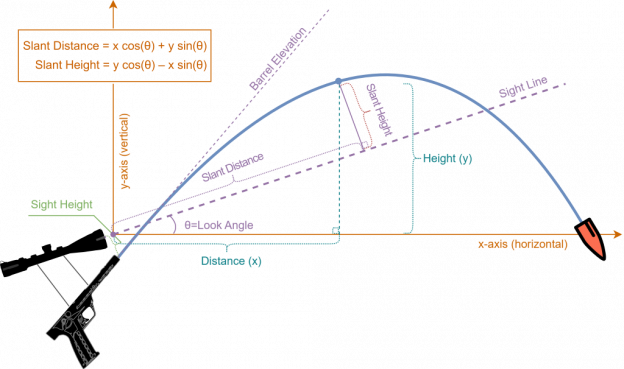
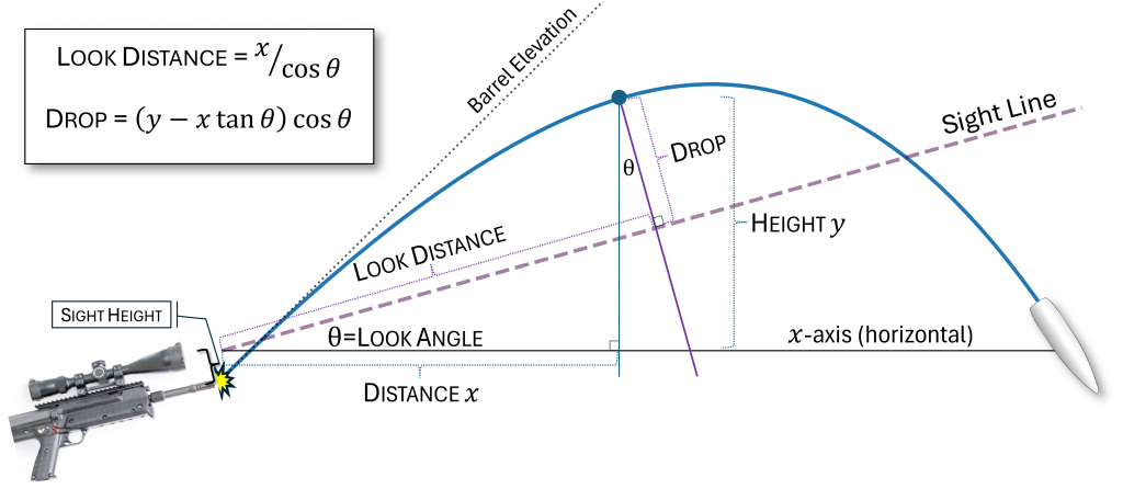
Graphic by David Bookstaber illustrating the trigonometry behind sight lines and ballistic trajectories.
Graphic I made to illustrate some of the concepts incorporated into the latest ballistic calculator.

While working on my ballistics book I got sidetracked building a ballistic calculator. I wanted to programmatically generate some examples, so 6 months ago I went to see what was available in open source. As I have noted previously, Python is preferred for this sort of hacking. I found this recently active Python project that looked promising and began to play with it. I encountered some bugs, noted them on GitHub, and was soon collaborating with the Ukrainian developer behind the project. Since then I have sporadically worked on adding features and improving the code in my fork here. These became quite extensive, and today we merged all of my work into his repository as a version 2 release!

One valuable feature set I added was to clearly handle non-zero look angles – i.e., when the shooter is sighting above or below the horizon. All useful ballistic calculators accept look angle as an optional parameter, but none that I have seen make it clear in their output if/when their distance and drop values are relative to the sight line or to the horizon.

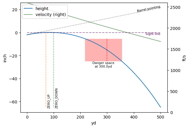
One of the plots generated by the calculator, highlighting danger space for a specific target and trajectory.

Technical details: The calculator simulates a ballistic trajectory using standard aerodynamic drag models together with a point-mass model of motion, sometimes referred to as 3 degree-of-freedom (3 DoF). It incorporates atmospheric variables, including multiple wind readings, as well as models of the change in air density by altitude over a trajectory. It adds Litz’s spin-drift approximation to windage, so I like to call it 3DoF+ since spin is another degree of freedom. (I don’t claim 4 degrees of freedom because the spin isn’t fully modelled. Amusingly, Hornady published a calculator under the trademark 4DOF® even though theirs likewise provides only auxiliary approximations of spin effects.)

Friction and muzzle velocity variation

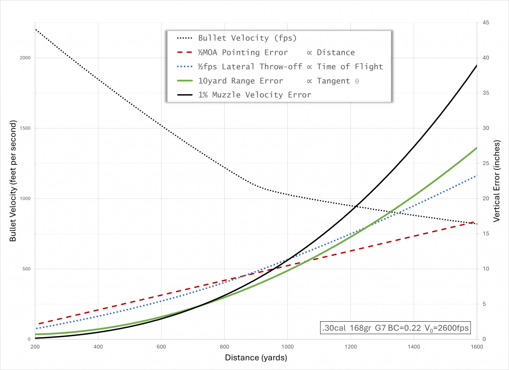
Minimizing muzzle velocity variance is a key to long-range shooting precision. The following chart (taken from my forthcoming book) shows the downrange effects of typical sources of vertical error in a typical .30 caliber rifle shot. In this example, the change in vertical impact caused by a 1% change in muzzle velocity is negligible at shorter ranges, but after 1000 yards it dominates the other sources of error:

Vertical change by distance from various sources of ballistic variation, shown for a typical 168gr .30 caliber rifle shot.

What causes muzzle velocity variance, and what can we do to reduce it? One obvious source is variation in powder charge weight. Within the range of safe powder charges, muzzle velocity shows a linear increase with the mass of powder. So precision loaders meter powder charge weights to hundredths of a grain. But even after eliminating any measurable variation in the weight and dimensions of cartridges, it is not uncommon to find the standard deviation of muzzle velocity running up to 1%.

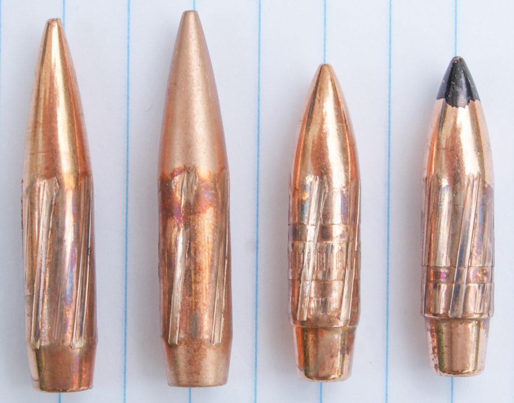
What else is there? Jeff Siewart has identified variation in engraving force1 as a significant source of variation in muzzle velocity. What is engraving? Here are pictures of bullets, before and after being fired through a rifled barrel:

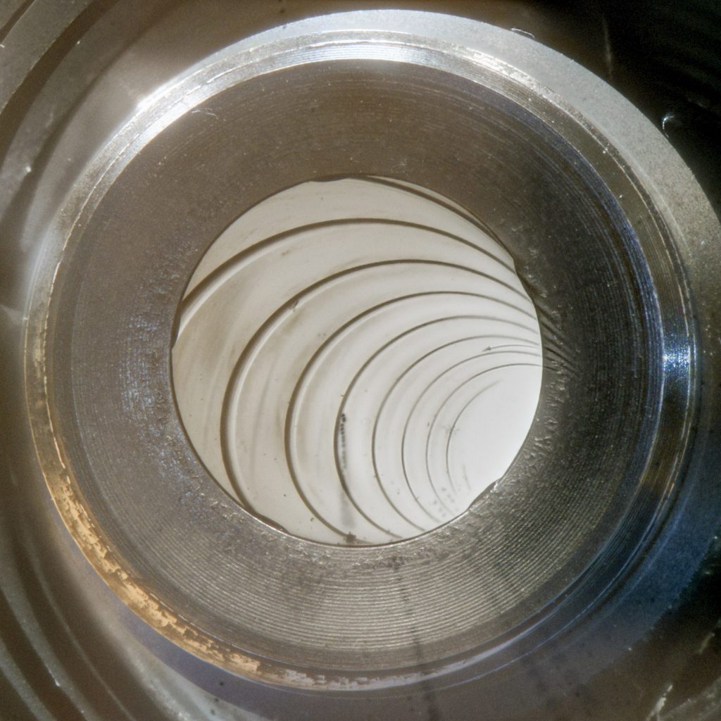
As a bullet enters a rifled barrel it has to engage and follow the rifling so that it gets spin stabilized. Engraving refers to the raised steel rifling of the barrel scraping into the surface of the bullet, as well as the entire circumference of the bullet deforming to create a tight seal with the barrel to keep the propellant gases from blowing past the bullet. Siewart has shown that the friction involved in engraving varies enough from one shot to another to cause the variations observed in muzzle velocity.

This engraving friction becomes even more significant in subsonic rifle rounds because (a) they are longer, which increases the surface area that must be engraved; and (b) they are fired at lower pressures and velocities, so the same variations in engraving force are a larger proportion of the total internal ballistic impulse.

Can we reduce friction?

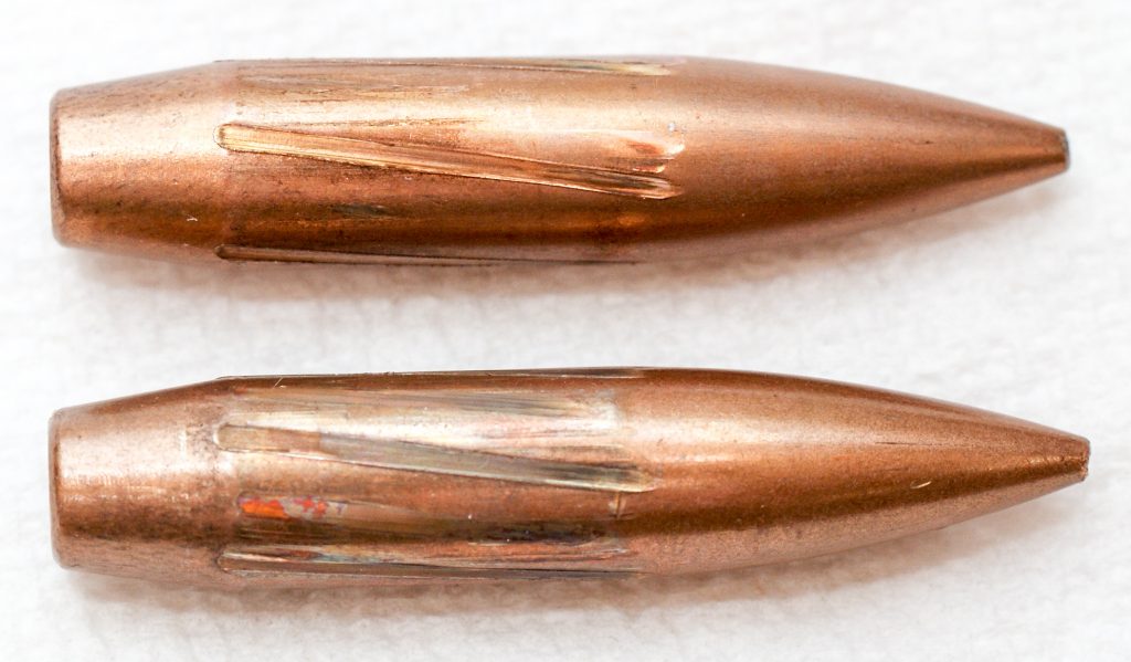
There are two established ways of reducing friction between bullet and bore. One is to reduce the bearing surface area of the bullet that contacts the barrel. A notable example of this approach was the addition by Barnes Bullets of cannelures to its solid copper bullet, which markedly increased its shooting precision.2 The following photo shows how these cannelures reduce the engraved surface area (as well as providing more relief for material displaced by engraving):

Barnes TSX solid copper bullet with cannelures to reduce and relieve engraved surface area

The other method of reducing friction is lubrication. Ten years ago I did extensive testing of various bullet and barrel lubricants in subsonic .30 bullets. Some of these did measurably reduce friction and improve shooting precision: Rydol’s “polysonic” treatment and Dyna-Tek’s “Nano-Ceramic” coating. Impact-plating with hBN (hexagonal boron nitride) did not. This is described in detail here. I didn’t test but would also expect the established MoS2 (“moly”) and WS2 (tungsten disulfide) bullet coatings to produce the same benefits.


1 See §Peak Engraving Pressure Variation, p.5 in November 2023 paper, “Using an Error Budget Approach to Estimate Muzzle Velocity Variation.”

2 See pp.4-6 in December 2020 paper, “What causes Dispersion.”

Freebore Boost in Rimfire Pistol

Longer gun barrels generally create higher velocities because they give a bullet more time to be accelerated by the propellant. (Detail post on the physics of this here.) Only in rimfire cartridges do we ever see the limit of this reached: After about 18″ of barrel a standard .22LR cartridge, which contains less than 1gr of powder, will start to decelerate as the friction of the bullet with the barrel exceeds the dwindling pressure produced by the small volume of propellant gas.

We’ve mentioned freebore boost before: This is the extra velocity that a bullet picks up passing through a suppressor. A suppressor is sort of a leaky barrel, so an inch of suppressor doesn’t boost velocity as much as an inch of barrel, but it can still add something. But does it provide boost even with the low propellant volumes seen in rimfire cartridges?

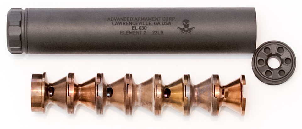
Here is a picture of the internals of a typical suppressor (here an Element 2 by AAC): It’s a series of baffles that vent the propellent into the enclosure as the bullet passes through. This .22 rimfire suppressor is just over 5″ long.

AAC Element .22LR Suppressor

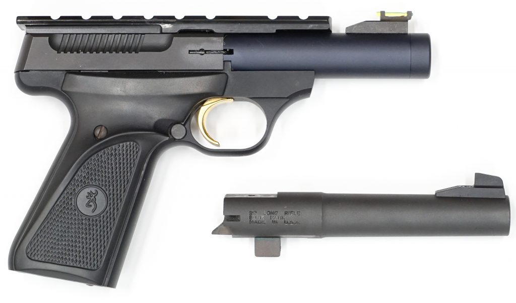
I chronographed shots through a Buckmark pistol in three configurations:

  1. 4″ barrel
  2. The same 4″ barrel with 5″ suppressor attached
  3. 5.5″ barrel
Buckmark .22LR Pistol with 4″ barrel (installed) and 5.5″ barrel

I tested two different cartridges: CCI SV (which has 0.6gr of powder behind a 40gr bullet) and Gemtech (which has 0.8gr of powder behind a 42gr bullet). Here are the results:

Cartridge4″ Bbl4″ bbl + 5″ suppressor5.5″ bbl
CCI SV883 ± 4.7 (n=30)904 ± 3.7 (n=69)930 ± 5.3 (n=30)
Gemtech897 ± 9.3 (n=20)907 ± 3.9 (n=55)941 ± 4.3 (n=30)
Muzzle Velocity in feet per second (fps), with 90% Confidence Intervals

In both cases the freebore boost was significant. With CCI SV ammo the suppressor added about half as much velocity as lengthening the barrel from 4″ to 5.5″. With Gemtech’s load it added a quarter as much.

Universal Precision Test Fixture for Firearms

I have spent a lot of time testing the precision of common firearms. As I have been explaining for years, it takes a lot of shots to get statistically significant measurements of precision. And I wanted to be able to collect large samples without wondering whether I as a shooter was introducing variance in the results.

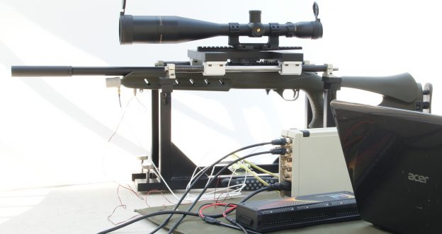
In order to remove the shooter from the equation, precision ballistics researchers going back as far as Franklin Mann in the late 1800s have used “V rests” to clamp barrels to benches.  I wanted to do the same, but with a wide variety of modern firearms, and without disassembling them. So ten years ago I built two “test rigs” with the following design objectives:

  1. Securely hold any gun with a scope rail;
  2. Allow the gun to be loaded, unloaded, and fired while attached;
  3. Precisely return the firearm to the same zero after every shot.

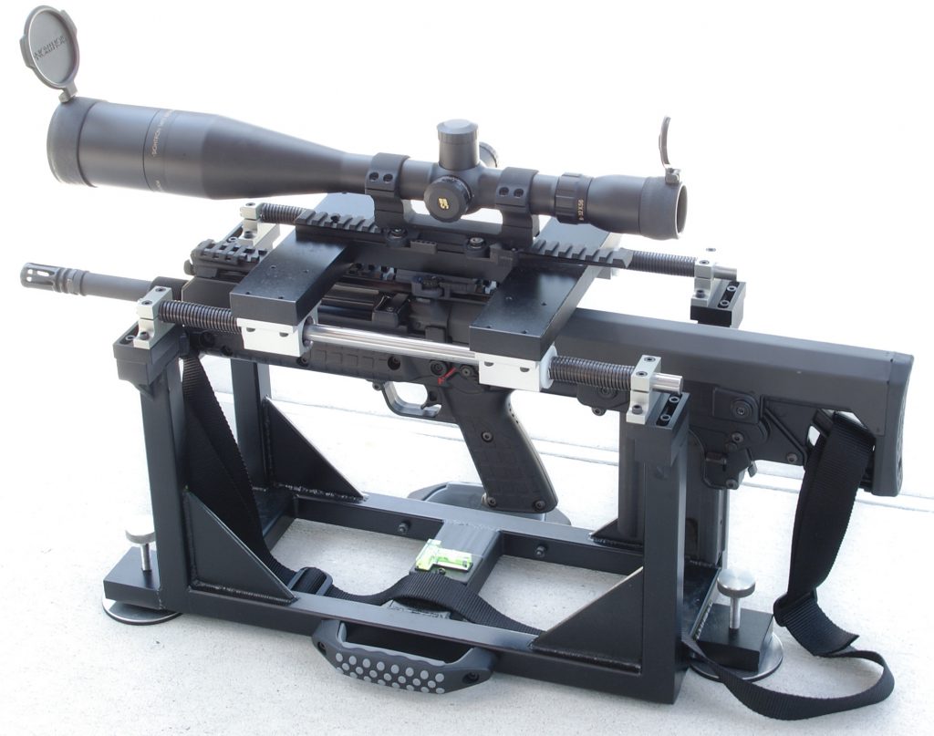
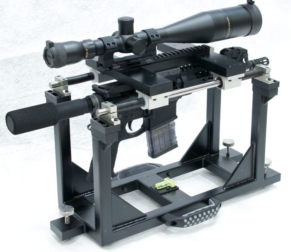
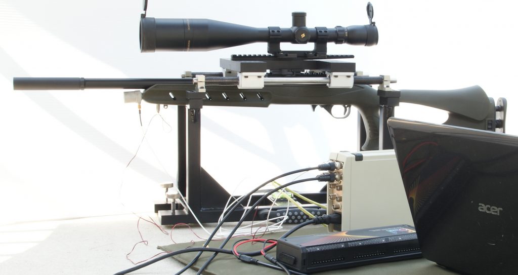
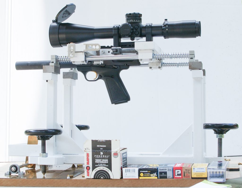
Here are photos of the first version:

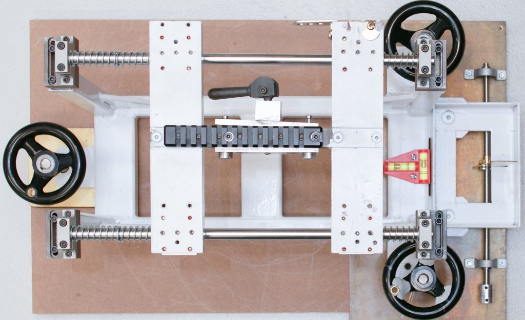
With a gun clamped in the fixture, I can precisely align it with the same point on the target for every shot, and then fire it while touching only the trigger. Both versions consist of:

  1. A Lower Frame supported on the bench with three Screws to fine-tune the point of aim.  To maximize their turning precision, the inserts use class 3 threads, and the end of each screw is turned to a sharp point.  The Lower Frame is tall enough to hold any man-portable gun with a magazine inserted.
  2. Two chrome-plated 12mm linear rail Shafts clamped to the Lower Frame.
  3. Two linear ball bearing Bushings on each Shaft.
  4. Springs that fit over the Shafts to absorb recoil of the Upper Bracket.
  5. An Upper Bracket, H-shaped, that screws into the Bushings.
  6. A Scope Rail on top of the Upper Bracket, to which I fixed a scope with up to 32x magnification.
  7. In the center of the Upper Bracket are two side Clamp Plates with a V channel cut along their length for gripping the scope rail of any gun to be tested.  One of the Clamp Plates rides on pins with springs, and is pushed by a Camming Lever to quickly clamp and release the guns.

The second version of the fixture added threads on top of the Upper Bracket for attaching up to 20 pounds of weight to dampen recoil, as well as a tray in the front that held up to 40 pounds of lead to keep it from lifting off the bench when shooting .308 rifles.

Target data from David Bookstaber

Statistical Inference Example: Testing .22LR Ammunition

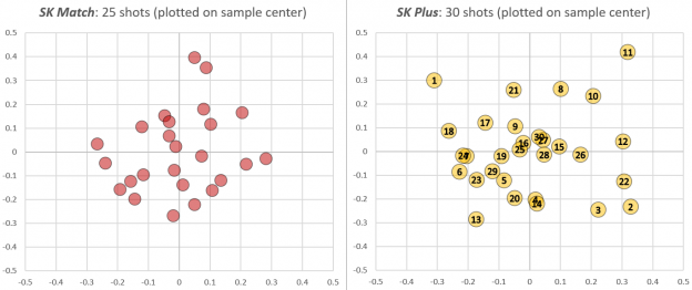
Competitive shooters work hard to find the ammunition that delivers the highest precision in their guns. This isn’t always straightforward: Even among premium ammunition lines any particular barrel can show a preference for one load that produces poor results in others. Using the latest statistical techniques, I plugged in some of the data I collected during this test of .22LR rifles. Shown here are the recorded groups of two types of ammunition – SK Plus and SK Match – shot through my KIDD 10/22.

Aggregated test targets shot through KIDD 10/22 at 50 yards. The SK Plus points are labelled in the order they were shot.

Match is SK’s higher-end ammunition, so our expectation going into the test is that it will produce higher precision than Plus. The purpose of the analysis here is to see how well a controlled test sustains that hypothesis.

I like to call this the Not So Fast! example. Remember that shooters never have enough time or ammunition, so they prefer to draw conclusions as fast as possible when running A/B tests like this. So imagine you have first fired the 25 round group of Match shown on the left. Running the calculations, you find its estimated sigma is 0.16″ at 50 yards with a 90% confidence interval of [0.13″, 0.19″].

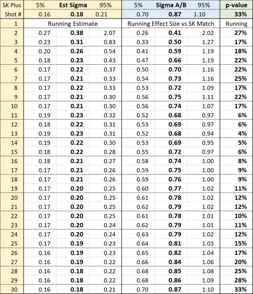
Now we want to see how SK Plus stacks up. In the following table I show how the statistics evolve with each shot of Plus:

Running statistics after each shot of SK Plus, compared to the complete target data of SK Match

The first few shots aren’t very good: by the third shot of Plus we estimate it is only half as accurate as Match: Sigma A/B = 0.50. (That’s the middle columns in the table: “Effect Size,” which is the ratio of the estimated sigma of the two ammo types.) But three shots is a terribly small sample, which is reflected in the very wide 90% confidence interval on that estimated Effect Size: [0.33, 1.27].

So we keep shooting, and Plus starts to look better. After 10 shots our estimate of its dispersion (a.k.a. sigma, which is the left three columns) has gone from over 0.3″ to barely over 0.2″. But compared to our data on Match it’s still not looking good: by the 11th shot the 90% confidence interval on Effect Size no longer contains 1.0, which means that with 90% probability it falls short of the precision of Match. This is also reflected in the p-value (right-most column), which collapses to single digits at this point.

But wait! We planned to shoot 30 rounds, so let’s finish the test. By the time we’ve fired 20 rounds of Plus we are not as confident that it is so inferior to Match. By the end of the test our best guess is that, in this gun, Match will produce groups only 15% tighter than Plus (that’s 1/0.87). And the probability of these aggregated data if there were no difference between the two (i.e., under the null hypothesis, which is the p-value) has jumped to 33%.

What’s the point?

  1. This example shows that small samples can suggest things that are far from the truth. We drew the worst samples of Plus right at the start of the test.
  2. By running a more statistically significant test, we have learned that when Match is scarce or expensive, we probably don’t give up much performance by instead shooting Plus through this rifle.

Excel file with the complete data and analysis is here.

Checking Probability and Statistics via Simulation

Did I get all these formulas right?

David Bookstaber's statistical formulae for Gaussian and Rayleigh parameter estimates and confidence intervals.

I’ve published the details on my Ballistipedia Github. I’ll explain how Monte Carlo simulation techniques enable anyone to verify whether these are correct. But first, the motivation:

Many shooting sports require relentless pursuit of precision in guns and ammunition. Amateur sportsmen spend thousands of dollars and hours a year trying to tweak their gear for marginal improvements in accuracy. Sadly, a lot of this effort is wasted because they lack an adequate understanding of probability and statistics.

Here is a common example: A shooter is tuning a load for a rifle. This involves assembling lots of ammunition in which the powder charge is varied by fractions of a grain over a range of acceptable values, then shooting the lots and seeing if any are exceptionally precise. But powder and bullets have become increasingly expensive, and each load and shot takes time, so there is constant pressure to draw conclusions from as few samples as possible. Compound this with the reality that humans are pattern-seeking machines who are so easily fooled by randomness that superstition is a hallmark of our species. Now we have legions of shooters going through the motions of experimentation but in the end making decisions based on essentially random noise.

As part of my renewed effort to apply rigorous statistical inference to amateur ballistics, I have been compiling formulas for p-values and confidence intervals on parameter effect size estimates for Gaussian, Exponential, and Rayleigh probability distributions.

When dealing with small samples there are bias correction terms that become increasingly relevant: For example, when n=3 failing to correct for bias leads to an estimate of standard deviation that is on average 20% too low! But how many degrees of freedom are involved? For a Rayleigh parameter estimate is it 2n, 2n-1, or 2n-2? Answer: When the samples are derived from bivariate normal coordinates where we have to estimate the center we give up two degrees, so the Gaussian correction term which is calculated with 2n+1 for a pure Rayleigh sample should be run with 2n-1, and the estimate itself is a chi-squared variate with 2n-2 degrees of freedom. How can I be certain I got that right?

This is one of the great things about fast computers and good (pseudo-) random number generators: We can actually resort to fundamental definitions and run simulations to verify statistical formulas. The definition of an x% Confidence Interval is a range of values that contains the true parameter in exactly x% of experiments. In the real world cases we care about we generally do not know the true parameter of a random variable with certainty. But when I programmatically generate a random number I know exactly what the parameter is, because I have to specify it. So with a random number generator we can simulate experiments in which we know the true parameter.

In the figure above I have formulas for confidence intervals. Are they correct? Here’s one way to check: I simulate many experiments using the random number generator, and in each experiment I use the formula to calculate a confidence interval. Then I just count how many times the confidence interval contains the true parameter. If my formula is correct, it will match the average I find through repeated experimentation. And the more simulations I run, the closer my average observation comes to the true value. (This is a fundamental theorem of probability called the Law of Large Numbers.) With modern computers I can run this simulation millions of times in a matter of seconds, which is enough to see these numbers converge to 4 or more significant figures.

My GitHub contains Jupyter notebooks where you can see and even re-run the code for these simulations. The statistics here are not extraordinary, and the formulas are widely known. More advanced statistical inference here includes some formulas that I could not find anywhere else.

Muzzle Velocity is Normally Distributed (+Infographic!)

I’m putting together a book with a lot of statistics applied to ballistics and trying to fill it with helpful examples since the pure math is hard to absorb. Below is one infographic I just finished. It’s an analysis of the muzzle velocity I measured shooting a full box of subsonic .22LR. The left column is all 50 measurements, which I then sort into a histogram to illustrate how muzzle velocity is normally distributed.

AR-15 buffers, springs, and cyclic rates

Animation of the AR cycle: Gas tapped from the barrel unlocks the bolt and pushes it rearward against a buffer and spring in the stock. During this travel it ejects the empty case and cocks the trigger. The recoil spring pushes the bolt assembly back into battery, and along the way the bolt strips a round from the magazine and pushes it ahead into the chamber.

Here is a good page describing the essential components and design considerations in an AR-15 action. In this post I summarize some research I did focusing on the tail end of the system: The recoil spring and buffer. In order to see exactly what goes on in there I cut a viewport into a buffer tube, clamped rifles into my test fixture, and recorded high-speed video of the action cycling.

Continue reading