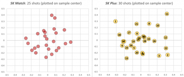
Competitive shooters work hard to find the ammunition that delivers the highest precision in their guns. This isn’t always straightforward: Even among premium ammunition lines any particular barrel can show a preference for one load that produces poor results in others. Using the latest statistical techniques, I plugged in some of the data I collected during this test of .22LR rifles. Shown here are the recorded groups of two types of ammunition – SK Plus and SK Match – shot through my KIDD 10/22.

Match is SK’s higher-end ammunition, so our expectation going into the test is that it will produce higher precision than Plus. The purpose of the analysis here is to see how well a controlled test sustains that hypothesis.
I like to call this the Not So Fast! example. Remember that shooters never have enough time or ammunition, so they prefer to draw conclusions as fast as possible when running A/B tests like this. So imagine you have first fired the 25 round group of Match shown on the left. Running the calculations, you find its estimated sigma is 0.16″ at 50 yards with a 90% confidence interval of [0.13″, 0.19″].
Now we want to see how SK Plus stacks up. In the following table I show how the statistics evolve with each shot of Plus:
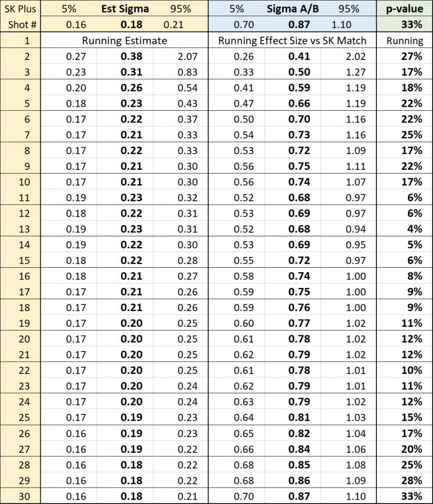
The first few shots aren’t very good: by the third shot of Plus we estimate it is only half as accurate as Match: Sigma A/B = 0.50. (That’s the middle columns in the table: “Effect Size,” which is the ratio of the estimated sigma of the two ammo types.) But three shots is a terribly small sample, which is reflected in the very wide 90% confidence interval on that estimated Effect Size: [0.33, 1.27].
So we keep shooting, and Plus starts to look better. After 10 shots our estimate of its dispersion (a.k.a. sigma, which is the left three columns) has gone from over 0.3″ to barely over 0.2″. But compared to our data on Match it’s still not looking good: by the 11th shot the 90% confidence interval on Effect Size no longer contains 1.0, which means that with 90% probability it falls short of the precision of Match. This is also reflected in the p-value (right-most column), which collapses to single digits at this point.
But wait! We planned to shoot 30 rounds, so let’s finish the test. By the time we’ve fired 20 rounds of Plus we are not as confident that it is so inferior to Match. By the end of the test our best guess is that, in this gun, Match will produce groups only 15% tighter than Plus (that’s 1/0.87). And the probability of these aggregated data if there were no difference between the two (i.e., under the null hypothesis, which is the p-value) has jumped to 33%.
What’s the point?
- This example shows that small samples can suggest things that are far from the truth. We drew the worst samples of Plus right at the start of the test.
- By running a more statistically significant test, we have learned that when Match is scarce or expensive, we probably don’t give up much performance by instead shooting Plus through this rifle.