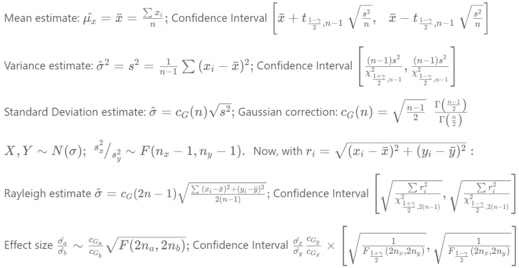
Did I get all these formulas right?

I’ve published the details on my Ballistipedia Github. I’ll explain how Monte Carlo simulation techniques enable anyone to verify whether these are correct. But first, the motivation:

Many shooting sports require relentless pursuit of precision in guns and ammunition. Amateur sportsmen spend thousands of dollars and hours a year trying to tweak their gear for marginal improvements in accuracy. Sadly, a lot of this effort is wasted because they lack an adequate understanding of probability and statistics.

Here is a common example: A shooter is tuning a load for a rifle. This involves assembling lots of ammunition in which the powder charge is varied by fractions of a grain over a range of acceptable values, then shooting the lots and seeing if any are exceptionally precise. But powder and bullets have become increasingly expensive, and each load and shot takes time, so there is constant pressure to draw conclusions from as few samples as possible. Compound this with the reality that humans are pattern-seeking machines who are so easily fooled by randomness that superstition is a hallmark of our species. Now we have legions of shooters going through the motions of experimentation but in the end making decisions based on essentially random noise.

As part of my renewed effort to apply rigorous statistical inference to amateur ballistics, I have been compiling formulas for p-values and confidence intervals on parameter effect size estimates for Gaussian, Exponential, and Rayleigh probability distributions.

When dealing with small samples there are bias correction terms that become increasingly relevant: For example, when n=3 failing to correct for bias leads to an estimate of standard deviation that is on average 20% too low! But how many degrees of freedom are involved? For a Rayleigh parameter estimate is it 2n, 2n-1, or 2n-2? Answer: When the samples are derived from bivariate normal coordinates where we have to estimate the center we give up two degrees, so the Gaussian correction term which is calculated with 2n+1 for a pure Rayleigh sample should be run with 2n-1, and the estimate itself is a chi-squared variate with 2n-2 degrees of freedom. How can I be certain I got that right?

This is one of the great things about fast computers and good (pseudo-) random number generators: We can actually resort to fundamental definitions and run simulations to verify statistical formulas. The definition of an x% Confidence Interval is a range of values that contains the true parameter in exactly x% of experiments. In the real world cases we care about we generally do not know the true parameter of a random variable with certainty. But when I programmatically generate a random number I know exactly what the parameter is, because I have to specify it. So with a random number generator we can simulate experiments in which we know the true parameter.

In the figure above I have formulas for confidence intervals. Are they correct? Here’s one way to check: I simulate many experiments using the random number generator, and in each experiment I use the formula to calculate a confidence interval. Then I just count how many times the confidence interval contains the true parameter. If my formula is correct, it will match the average I find through repeated experimentation. And the more simulations I run, the closer my average observation comes to the true value. (This is a fundamental theorem of probability called the Law of Large Numbers.) With modern computers I can run this simulation millions of times in a matter of seconds, which is enough to see these numbers converge to 4 or more significant figures.

My GitHub contains Jupyter notebooks where you can see and even re-run the code for these simulations. The statistics here are not extraordinary, and the formulas are widely known. More advanced statistical inference here includes some formulas that I could not find anywhere else.